Global fire activity: weekly data and a continuous-domain reconstruction

Left of the line: the weekly number of satellite fire detections, counted on the 2° grid the model was fitted to. Right of the line: the reconstruction, a function of continuous position on the sphere and of the time of year. Drag the line to compare the two; drag the slider to move through the 1,200 weeks from 2003 to 2025. Click anywhere on the map to see the fire season of that 2° cell below.

For rough spatio-temporal data, ℓ₁ regularization is a viable alternative to Gaussian processes: sparse, sharp, and open to any kind of measurement.

The content of the poster, section by section; click a title to open or close it.

1. Fire detections as measurements of a seasonal field

Many quantities on Earth repeat every year: fires, CO₂, temperature, epidemics. The unknown is a field f(s, t), with s on the sphere 𝕊² and t on the yearly circle 𝕋, which we only see through M linear measurements

y_{m} = ⟨ ν_{m}, f ⟩ + σ^{2} ε_{m}, ⟨ ν_{m}, f ⟩ = \int_{𝕊^{2} \times 𝕋} f (𝐬, t) d ν_{m} (𝐬, t),

where ε_m is noise and the sensor ν_m is a bounded measure: a point sample, the average over a cell, the total over a time window. Goal: recover f as a continuous function of space and time, from any kind of measurement.

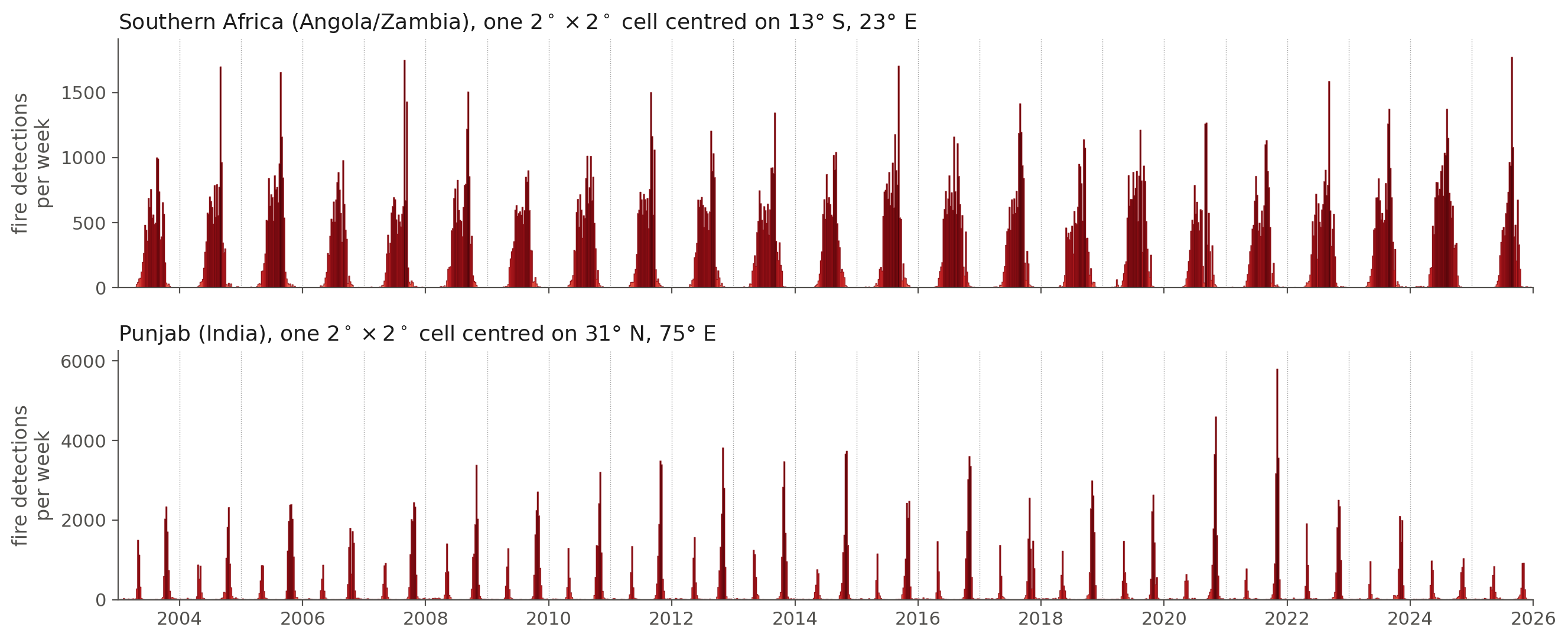
The fire data. NASA FIRMS active-fire detections (MODIS, 2003–2025), counted per week on 2° cells: 23 years × 52 weeks × 6005 land cells.

Weekly fire detections from 2003 to 2025 in two 2-degree cells: a yearly repetition of variable intensity — Weekly fire detections 2003–2025 in two 2° cells.

Fire formulation. Detections form a Poisson point process on 𝕊² × 𝕋 of unknown intensity f ≥ 0 (detections per unit area and time), so the count of the land cell C_m in the week W_m′ is a local integral of f:

y_{m m^{'}} \sim Poisson (⟨ ν_{s, m} \otimes ν_{t, m^{'}}, f ⟩), ⟨ ν_{s, m} \otimes ν_{t, m^{'}}, f ⟩ = \int_{C_{m}} \int_{W_{m^{'}}} f (𝐬, t) d t d 𝐬 .

The sensor is separable: a cell on the sphere times a week on the circle. Since f is one-year periodic, the 23 years of the same week share the same intensity. With the Poisson loss E(y, z) = z − y ln z, the data term of the problem below is the negative log-likelihood of the counts and its solution is the maximum a posteriori estimate of f.

2. Why not a Gaussian process? The limits of the L₂ approach

The classical answer is a Gaussian process (kriging): its posterior mean is also the minimiser of a quadratic, L₂-type penalty. With a separable covariance g_s(⟨s, ·⟩) g_t(t − ·), the GP posterior mean is

f_{GP} = \sum_{m = 1}^{M} b_{m} ψ_{m}, ψ_{m} (𝐬, t) = ⟨ ν_{m}, g_{s} (⟨ 𝐬, \cdot ⟩) g_{t} (t - \cdot) ⟩,

𝐛 = {(𝐊 + σ^{2} 𝐈)}^{- 1} 𝐲, 𝐊_{m m^{'}} = ⟨ ν_{m}, ψ_{m^{'}} ⟩ .

One atom ψ_m per measurement, and an M × M system to solve.

Ideal sampling, ν_m = δ at (s̄_m, t̄_m): the classical kriging formula, a shifted covariance, $ψ_{m} = g_{s} (⟨ \cdot, {\bar{𝐬}}_{m} ⟩) \otimes g_{t} (\cdot - {\bar{t}}_{m}) .$
General measurements (cell and window averages): no closed form, $ψ_{m} (𝐬, t) = \iint g_{s} (⟨ 𝐬, 𝐬^{'} ⟩) g_{t} (t - t^{'}) d ν_{m} (𝐬^{'}, t^{'}) :$ every atom is a double integral of the covariance against its sensor, to be computed numerically for each of the M measurements before the system can even be formed.

Whatever the sensors, the GP solution is a sum of M atoms that are all as smooth as the covariance: nothing in it is sparse, and sharp seasonal features are smoothed out. Lessons from compressed sensing: use the ℓ₁ norm to promote solutions that are sparse in a given dictionary.

3. The continuous-domain model: an optimization problem

The field splits into a seasonal cycle (zero mean over the year) and a yearly mean, f = f_cycle + f_mean(s). We solve

\min_{f} \underset{fit to the data}{\underset{⏟}{\sum_{m = 1}^{M} E_{m} (y_{m}, ⟨ ν_{m}, f ⟩)}} + λ \underset{few seasonal changes}{\underset{⏟}{{‖ [L_{s} \otimes \partial_{t}^{n}] {f_{cycle}} ‖}_{𝓜}}} + λ_{0} \underset{simple yearly mean}{\underset{⏟}{{‖ L_{s} {f_{mean}} ‖}_{𝓜}}} .

∂_tⁿ measures changes along the year (n = 4 in the fire fits); L_s measures roughness on the sphere.
The 𝓜-norm (the total variation of a measure) is the measure-theoretic extension of the ℓ₁ penalty: it asks for few seasonal changes and a simple yearly mean rather than for small ones everywhere.

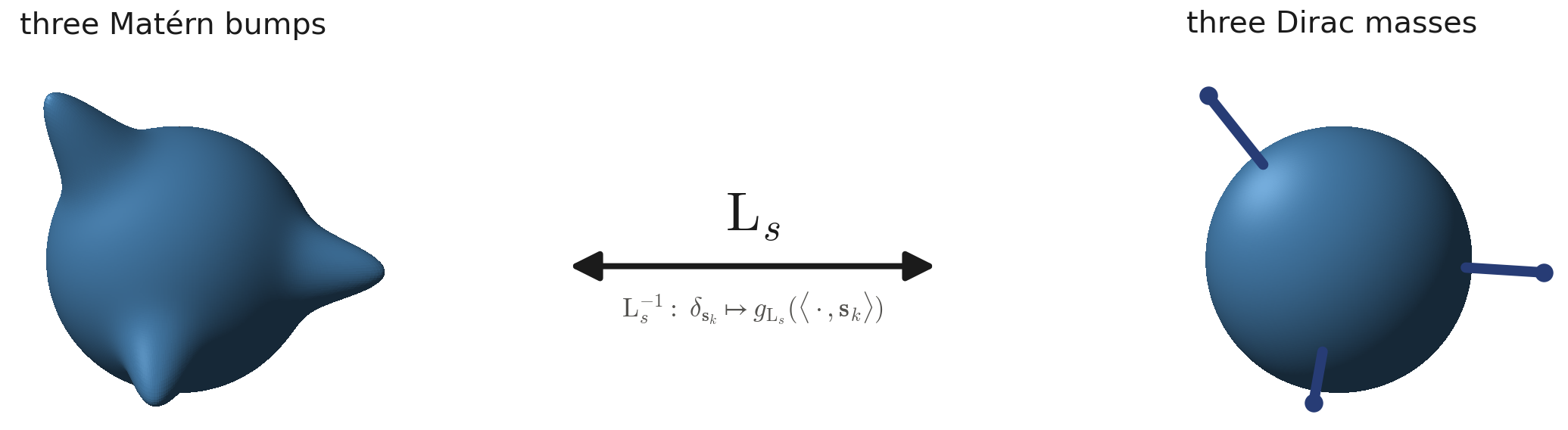
Two spheres: the spherical operator L_s applied to a bump, and its Green's function — The spherical operator L_s and its Green's function g_{L_s}.

4. The shape of the solutions: a representer theorem

Theorem (representer). The extremal solutions of the problem of section 3 are spatio-temporal splines:

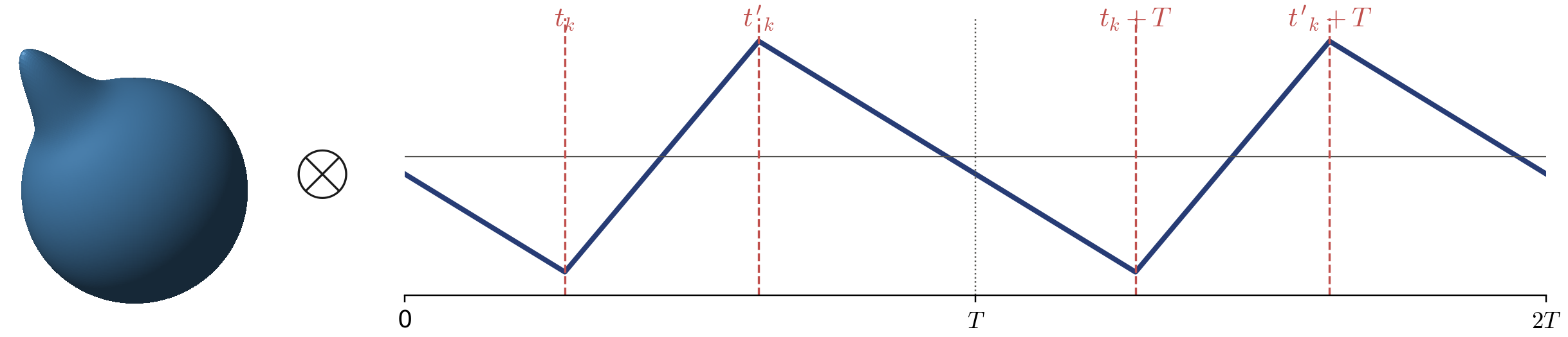
f^{⋆} = \sum_{k = 1}^{K_{1}} a_{k} \underset{bump on the sphere}{\underset{⏟}{g_{L_{s}} (⟨ \cdot, 𝐬_{k} ⟩)}} \otimes \underset{a change at t_{k}, undone at t_{k}^{'}}{\underset{⏟}{(g_{n} (\cdot - t_{k}) - g_{n} (\cdot - t_{k}^{'}))}} + \sum_{k = 1}^{K_{0}} c_{k} \underset{yearly mean}{\underset{⏟}{g_{L_{s}} (⟨ \cdot, 𝐬_{0, k} ⟩)}},

with fewer unknowns than data: K₁ + K₀ ≤ M. Here g_{L_s} is the Green's function of L_s and g_n that of ∂_tⁿ on the circle, so that g_n(· − t_k) − g_n(· − t′_k) is a change of the seasonal level that starts at t_k and is undone at t′_k.

Atoms are products of shifted Green's functions: a bump on the sphere times a change along the year.
Holds for any linear measurement (averages, point samples).

One atom of the solution: a bump on the sphere times a change along the year — One atom of the solution.

5. Discretization and the computed solution

Discretization. Restrict the parameters of the representer formula to a grid:

f_{𝐀} (𝐬, t) = \sum_{k = 1}^{K_{Ξ}} \sum_{k^{'} = 1}^{K_{T}} 𝐀 [k, k^{'}] g_{L_{s}} (⟨ 𝐬, 𝐬_{k} ⟩) β_{n, h} (t - h k^{'}),

where A is the coefficient matrix (one row per bump, one column per knot of the year), g_{L_s}(⟨·, s_k⟩) the bump centred at s_k, and β_n,h the periodic B-spline of degree n − 1 with knot spacing h. Setup: for separable measurements ν_s,m ⊗ ν_t,m′ the problem of section 3 is exactly

\min_{𝐀} \sum_{m, m^{'}} E_{m m^{'}} (y_{m m^{'}}, {[𝐒^{⊤} 𝐀 𝐓]}_{m m^{'}}) + λ h^{n - 1} {‖ 𝐀 * 𝐝_{n} ‖}_{1} + λ_{0} {‖ \bar{𝐚} ‖}_{1},

where

$𝐒 [k, m] = ⟨ ν_{s, m}, g_{L_{s}} (⟨ \cdot, 𝐬_{k} ⟩) ⟩$ : the bump k seen by the spatial sensor m (the integral of the bump over the cell C_m);
$𝐓 [k^{'}, m^{'}] = ⟨ ν_{t, m^{'}}, β_{k^{'}} ⟩$ : the B-spline k′ seen by the time sensor m′ (its integral over the week W_m′);
$𝐝_{n}$ : the n-th periodic finite differences, so that $𝐀 * 𝐝_{n}$ lists the seasonal changes of every bump;
$\bar{𝐚} = 𝐀 𝟏 / K_{T}$ : the yearly mean of each bump's coefficients.

Solve with a primal-dual splitting (here ADMM). Fast because S and T are small and sparse: a bump overlaps a handful of cells, a B-spline a handful of weeks.

The fire fits.

Space: K_Ξ ≈ 39,000 Matérn bumps g_{L_s} (smoothness 5/2, scale 0.52°, width at half maximum 1.1°) centred on a Fibonacci lattice where they reach land. Time: K_T = 52 cubic periodic B-splines, one per week (n = 4, h = one week).
Coefficients A ≥ 0: the intensity is nonnegative.
λ₀ = 10⁻³ λ; λ = 6.8·10⁻³, chosen on 10 % held-out data at a coarser scale (0.63° bumps) and rescaled by the ratio of the bumps' masses.

What the map shows: an approximate solution. Because the atoms sit on a fixed grid instead of free positions, and the iterations run to a finite accuracy, f_A is an approximation of the solution of the continuous-domain problem. It is the function drawn to the right of the line, evaluated at every pixel and averaged over the selected week.

◀ 2° weekly data continuous reconstruction (𝓜) ▶

◀▶

Loading…

fire detection density / week

6. Results on the poster: 𝓜-norm against L₂

The poster fits the same problem twice, with the 𝓜-norm penalty shown on the map and with its quadratic (L₂) counterpart, at the same budget.

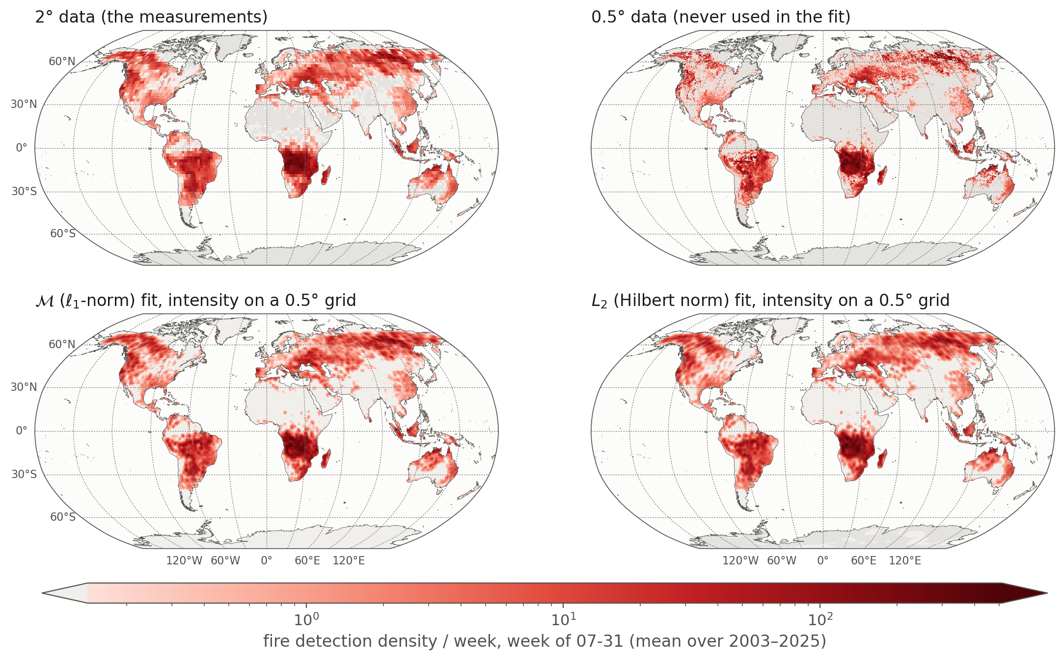
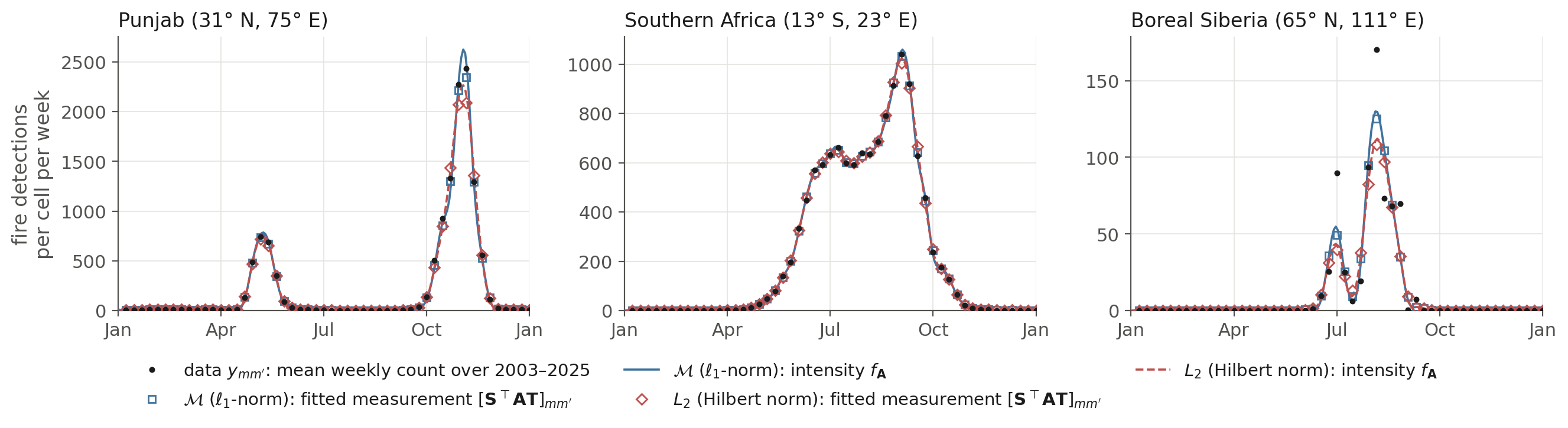
Four maps of a week of late July: the 2-degree data, the 0.5-degree data, the M-norm reconstruction and the L2 reconstruction — A week of late July. Fitted on 2° cells, the models recover structure at 0.5°: log-RMSE against the fine data 0.27, vs 0.29 for the 2° data itself.

Seasonal cycles at three cells: the folded weekly data, the M-norm fit and the L2 fit — Seasonal cycles at three cells.

The 𝓜-norm describes a bump's year with 13 changes out of 52 weeks; L₂ needs 36.
Both penalties predict unseen weeks equally well.
The 𝓜-norm keeps the short, intense seasons sharper.
Extends to a seasonal–trend decomposition.

References. V. Guillemet, J. Fageot, M. Unser, Spatio-temporal trend-seasonal decomposition: from ideal sampling to general measurements, preprint 2026 · M. Unser, J. Fageot, J. P. Ward, Splines are universal solutions of linear inverse problems with generalized TV regularization, SIAM Review 2017 · M. Simeoni, Functional penalised basis pursuit on spheres, ACHA 2021.

Data: NASA FIRMS, MODIS Collection 6.1 active-fire detections, counted per week on 2° land cells (2003–2025). Model: the 𝓜-norm (ℓ₁) penalised fit on the sphere × a periodic year, built from about 39,000 Matérn bumps and periodic cubic splines; on the map it is evaluated at every pixel and averaged over the selected week. It is the same every year: it describes the typical fire season. Colours as on the poster Sparse Spatio-Temporal Models on the Sphere for Seasonal Data Analysis (V. Guillemet, J. Fageot, M. Unser; SIAM Conference on Imaging Science 2026).